This page contains information related to my 2004 DPS abstract.

Abstract
Radio Wavelength Observations of Titan with the VLA
B.J. Butler NRAO
M.A. Gurwell CfA
Radio wavelength observations of Titan are a powerful technique for
probing through the atmosphere to the surface and subsurface. For
more than 20 years, the VLA has been used to observe Titan at
wavelengths from 0.7cm to 6cm. A synopsis of these observations
will be presented. Three results in particular will be focused on.
First, in 1992 seventeen short observations at 3.5cm were used to
create a radio light curve for Titan. Preliminary reduction of that
data showed no believable light curve (Grossman & Muhleman 1992, BAAS, 24, 954). New reduction,
including incorporation of sophisticated algorithms for removing
confusing sources (including Saturn), shows a detectable light curve,
peaking around 180o longitude, with a peak-to-peak
amplitude of ~10%. The mean brightness temperature of 79.3 +- 2.4 K
(including absolute uncertainty) is consistent with that found from
the earlier reduction. Second, in 1993 two long observations were
performed in an attempt to directly measure the dielectric constant
of the surface. The result from those experiments is a dielectric
constant of 2.7 +- 1.7. Third, in 1999 three long observations were
performed at 0.7cm in an attempt to detect C3H2 in the atmosphere.
As a byproduct of these observations, brightness maps at 0.7 and
1.3cm were produced - the highest resolution radio maps of Titan ever
made (~0.2"). These and other results will be presented.
Introduction
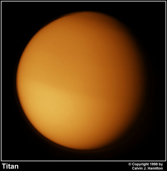
What is on the surface of Titan? When the Voyager spacecraft passed
by in 1980, it could not see the surface, due to obscuration by a
thick haze (see, e.g., this
description and Smith
et al. 1981, Science, 212, 163).
Atmospheric sensing instruments did, however, measure relatively
large amounts of methane (CH4) in the atmosphere
(Hanel
et al. 1981, Science, 212, 192). Although methane had been
seen in Titan's atmosphere as early as 1944
(Kuiper
1944, ApJ, 100, 378), the abundance was poorly known. The
Voyager results placed it at a few percent by fraction. While this
is a relatively small amount, it is too large a fraction to be
supported over long timescales because it would be photodissociated
too quickly. A source for methane must therefore exist. It was
suggested that a global ethane/methane liquid ocean could exist on
the surface which would supply the methane to the atmosphere
(Lunine,
Stevenson, & Yung 1983, Science, 222, 1229). It had to be
thick, though (of order 1 km), because an ocean of less than ~400
meters depth would provide too much tidal dissipation to allow for
the current eccentricity of the orbit of Titan
(Sagan
& Dermott 1982, Nature, 300, 731).
How could this hypothesis be tested? Observations of the surface
were needed, but it was clear that at optical wavelengths the surface
was completely obscured, at the time the near-IR windows (see below)
were not known, and further into the IR the observing facilities were
inadequate. Radio wavelengths (anything longer than a few mm),
however, easily penetrate through the haze and atmosphere to the
surface and were therefore considered a primary observational tool
for understanding the surface of Titan. Because the reflective (or
emissive, for passive work) properties of a solid (ice) surface would
be quite different from those of a hydrocarbon liquid surface, if
sensitive radio or radar observations could be made, the two types of
surfaces could be distinguished.
In 1989, radar echoes were first successfully obtained from Titan,
using the combined Goldstone/VLA
radar. The results were completely consistent with an icy surface -
i.e., the radar echoes were similar to what we had seen from the
Galilean satellites
(Muhleman
et al. 1990, Science, 248, 975;
Muhleman,
Grossman, & Butler 1995, AREPS, 23, 337).
A global, kilometers-deep methane/ethane ocean was completely ruled
out by these observations. However, variations were seen in the
radar echoes which were hard to understand in the context of a
normal icy surface - could there be ethane/methane "lakes" or "seas"
present? Dynamically it was possible
(Dermott
& Sagan 1995, Nature, 374, 238). In addition, there was early
indication from near-IR observations that it might be possible.
In the early 1990's it became apparent that at some wavelengths in
the near-IR the surface was being sensed and that the surface was
heterogeneous
(Lemmon,
Karkoschka, & Tomasko 1993, 103, 329;
Griffith
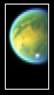
1993, Nature, 364, 511). Then, in 1995, HST provided the first
resolved images of the surface through one of these windows
(Smith
et al. 1996, Icarus, 119, 336).
It was suggested that the "bright" (in fact the contrast is only of
order 10%) areas were highlands ("continents") which had exposed ice,
washed clean by hydrocarbon rain. The dark regions were
ethane/methane ocean.
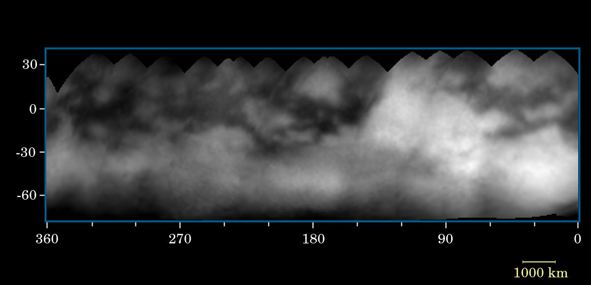
Since these early observations, there have been higher resolution
near-IR images made with speckle and AO techniques, including those
from La Silla/ADONIS (Combes et al. 1997), Keck (Gibbard et al.
1999; Brown, Bouchez & Griffith 2002; Roe et al. 2002; Gibbard et al.
2004), Gemini (Roe et al. 2002), CFHT (Coustenis et al. 2001), and
the VLT
(Hartung
et al. 2004 - image shown below).
With Cassini now in the Saturn system, it has started to send back
some spectacular images of Titan, including this one:
and this map:
It will only get better as Cassini takes more and higher resolution
images of Titan, and sends back a wealth of other data, including
radar and radio observations.
Further evidence for the existence of liquid hydrocarbon
was provided by recent radar observations from the upgraded
Arecibo radar
(Campbell
et al. 2003, Science, 302, 431). These observations show a
"specular glint" present in a large fraction of the echoes. This
could be the result of liquid lakes or seas.
Before the near-IR and more recent radar results were in hand, there
were attempts to measure the passive radio emission properties of
Titan. Similar to the radar experiments, such observations could be
used to discriminate between liquid ethane/methane and solid ice
(because of the different dielectric constants, and hence
emissivities, of the two types of surfaces). They still have
intrinsic value, as they are obtained over a wide wavelength range,
and hence sample different surface and subsurface size and depth
scales. The purpose of this work is to review those observations
and present results from them.
Instrument
The observations were all done at the
Very Large Array (the VLA is
operated by the National Radio
Astronomy Observatory, a facility of the
National Science Foundation
operated under cooperative agreement by
Associated Universities, Inc.),
which is a collection of 27 radio antennas spread out on the plains
of San Augustin, New Mexico.
1992 Light Curve Results
In February of 1992, Arie Grossman and Dewey Muhleman used the VLA
to observe Titan at X-band (effective frequency of 8.616 GHz)
on 17 different days (each observation was about 1 hour). The
intent was to see if there was a variation in the light curve, which
would be further indication of the possible presence of liquid
ethane/methane lakes or seas postulated at that time, or at least of
surface variations. Data reduction at that time showed no
statistically significant variation as a function of longitude, and
derived a value for the brightness temperature of 80.4 +- 0.6 K
(statistical error only - there is a 3% absolute uncertainty from
the flux density scale), implying a surface dielectric of 2.9 +- 0.6
when combined with other radio wavelength observations
(Grossman
& Muhleman 1992, BAAS, 24, 954).
I have re-reduced all of this data, taking advantage of new routines
to handle planetary motion and confusing source subtraction within
the AIPS package (in
which all of the reduction was done). The data reduction steps which
are above and beyond normal include:
- distance correction for the changing distance
during the 17 days (see
Butler
& Bastian 1999, SIRA II, ASP Conf. Ser. equations 31-19
through 31-21) - all of the data were modified as if the distance
was 10.9 AU;
- wave curvature correction (see Butler & Bastian 1999, equations
31-5 and 31-6);
- subtraction of Saturn as a confusing source, including the
proper phase modification to account for the differential motion
of Saturn (see Butler & Bastian 1999, equations 31-3 and 31-4),
and the changing primary beam response;
- subtraction of other background confusion sources, including
the proper phase modification to stop the motion of the
background sources;
- least squares fit of visibilities to get flux density (task
OMFIT in AIPS);
- conversion to brightness temperature (see Butler & Bastian
1999, equation 31-8).
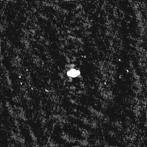
A final image is made to check the flux density fitted from the
visibilities. These images can be combined, after shifting the
data so that Saturn is in the field center (via the same phase
shifting technique referenced above), to make a combined image
where it appears that Titan is orbiting around Saturn (in reality,
since we observe with Titan at the field center, if we just
combined the images with no phase shift to get Saturn at the phase
center, it would appear as if Saturn were rotating around Titan).
The following table gives the relevant results:
| |
Date in 1992 |
|
Sub-Earth longitude |
|
flux density (mJy) |
|
brightness temperature (K) |
|
| |
Feb 01 |
|
76.1 |
|
1.31 +- .03 |
|
76.3 +- 1.7 |
|
| |
Feb 02 |
|
99.5 |
|
1.36 +- .03 |
|
79.0 +- 1.7 |
|
| |
Feb 03 |
|
124.5 |
|
1.39 +- .04 |
|
80.7 +- 2.2 |
|
| |
Feb 04 |
|
146.1 |
|
1.47 +- .04 |
|
85.1 +- 2.2 |
|
| |
Feb 07 |
|
211.2 |
|
1.34 +- .04 |
|
77.7 +- 2.2 |
|
| |
Feb 08 |
|
234.8 |
|
1.39 +- .03 |
|
80.5 +- 1.7 |
|
| |
Feb 09 |
|
258.1 |
|
1.31 +- .04 |
|
76.0 +- 2.2 |
|
| |
Feb 13 |
|
347.4 |
|
1.40 +- .04 |
|
81.0 +- 2.2 |
|
| |
Feb 15 |
|
29.9 |
|
1.28 +- .03 |
|
74.2 +- 1.7 |
|
| |
Feb 16 |
|
53.8 |
|
1.32 +- .03 |
|
76.3 +- 1.7 |
|
| |
Feb 17 |
|
76.7 |
|
1.32 +- .02 |
|
76.2 +- 1.1 |
|
| |
Feb 18 |
|
99.9 |
|
1.42 +- .03 |
|
81.7 +- 1.7 |
|
| |
Feb 20 |
|
144.3 |
|
1.50 +- .04 |
|
85.9 +- 2.2 |
|
| |
Feb 23 |
|
211.5 |
|
1.40 +- .04 |
|
80.1 +- 2.2 |
|
| |
Feb 25 |
|
256.5 |
|
1.40 +- .04 |
|
80.0 +- 2.2 |
|
| |
Feb 27 |
|
301.2 |
|
1.31 +- .04 |
|
74.9 +- 2.2 |
|
| |
Feb 29 |
|
345.0 |
|
1.28 +- .04 |
|
73.1 +- 2.2 |
|
| |
Mean (weighted) |
|
--- |
|
1.356 +- 0.014 |
|
78.3 +- 0.8 |
|
Note that the uncertainties here are only statistical. In absolute
terms, there is a roughly 3% uncertainty in the flux density scale
(derived using 3C286 in this case) which dominates the uncertainty
in the final flux density and brightness temperature.
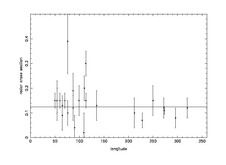
Here is a plot of the data (where observations are at two very near
longitudes, I have combined them - I've also added one of the
data points from the 1993 observations [see below] as the filled
triangle).
A sinusoidal fit is a decent representation to the data, and is
shown on the plot above - it peaks around 180 deg and has a
peak-to-peak amplitude of 8 K. This peak-to-peak variation is much
larger than the error on the measurements (it's about 20-sigma when
compared to the combined noise on the data), so is real. This is
mildly consistent with the radar results, which show a modest peak
in reflectivity around 90 deg - high reflectivity means low
emissivity, and a minimum in the radio brightness. But, in fact,
we expect a direct anti-correlation, and we do not see that (we
expect to be 180o out of phase, and we are
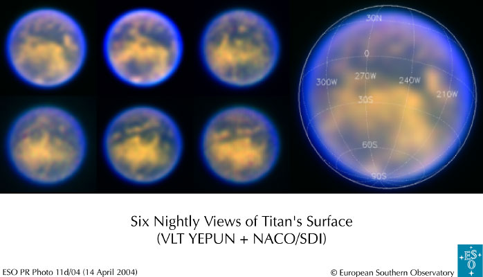
90o out of phase). This is also consistent with the
infrared albedo maps, which show the darkest regions from
150o to 330o and the brightest at the other
longitudes - here is the map from the recent ESO/VLT results (see
also the Cassini map above):
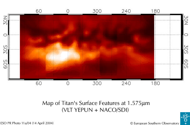
Bright regions are expected to be colder - both because they
reflect more incoming sunlight and because they may be higher,
topographically. Since they are colder, they will also appear so
in the radio (which is a combination of physical temperature and
emissivity). If they are ice, and the darker regions are
hydrocarbon liquid, then the variation is even more pronounced, as
the hydrocarbon has lower dielectric and hence higher emissivity.
So these results are in good agreement with the IR albedo results.
A model has been constructed which accounts for the radiation from
the surface and atmosphere of Titan (with a crude subsurface
contribution) - similar to that constructed for Venus
(Icarus 2001, 154, 226).
The important inputs to the model are the values of temperature,
total pressure, and fraction of CH4 and Ar, all as a
function of altitude in the atmosphere. The absorption in the
atmosphere is calculated by scaling the pure N2
absorption via (see Gurwell & Muhleman 1995, Icarus, 117, 375):
k = kN2 fN2
(1 + 3 fCH4)
where kN2 is the pure N2
absorption given in Dagg et al. 1975, Can. J. Phys., 53, 1764 (but
see also Courtin 1988, Icarus, 75, 245
and Borysow & Frommhold 1986, ApJ, 311, 1043),
and fN2 and fCH4 are
the fractions of N2 and CH4 in the
atmosphere. An equatorial surface temperature of 93.9 K is used,
with vertical profile given in
Lellouch et al. 1989, Icarus, 79, 328.
We use an equator to pole surface temperature difference of 13.5 K
(this matches the observed 4 K difference from equator to
60o latitude observed in the Voyager IRIS data - see Lorenz
et al. 2003, 51, 353;
Courtin
& Kim 2002, P&SS, 50, 309;
Samuelson
et al. 1997, P&SS, 45, 959).
We use a methane abundance of 4% at the surface
(Lemmon, Smith, & Lorenz 2002, Icarus, 160, 375),
with vertical profile given in Lellouch et al. 1989. We use an
argon abundance of 4%
(Gladstone et al. 2002, BAAS, 34, 902),
constant with altitude. We then run the model with varying values
of surface dielectric (using a smooth dielectric sphere for the
planet surface), in order to fit the surface dielectric given the
observed brightness temperature.
For the observed geometry (the Sub-Earth latitude, 20o
at the time, makes a difference because of the equator-to-pole
temperature variation), the mean brightness temperature results in
an effective dielectric constant of 3.2 +- 0.3 (3.2 +- 0.8 taking
into account the flux density scale uncertainty).
Results:
- dielectric = 3.2 +- 0.3 (formal uncertainty only)
dielectric = 3.2 +- 0.8 (absolute uncertainty included)
- Light curve of 10% - peaks at 185o longitude
1993 Surface Dielectric Results
One way of overcoming the uncertainty in the flux density scale and
how it propagates into uncertainty on the derived dielectric
constant is to take polarimetric measurements with an
interferometer. Such measurements are insensitive to overall flux
density scale offsets, since for the polarized quantity of interest
(from which the surface dielectric can be derived) the total flux
density is divided out (see the discussion in
Butler
& Bastian 1999, SIRA II, ASP Conf. Ser. Appendix A and
references therein).
In February of 1993, Arie Grossman and Dewey Muhleman used the VLA
to observe Titan at X-band (effective frequency of 8.616 GHz)
on 2 different days (one at each elongation) in 10-hour long tracks
in an attempt to do this. These observations were never published
(or even reduced), so the reduction I have done is completely new.
In fact, this is a very difficult measurement, since the polarized
flux density is of order a few percent of the total flux density,
which for Titan is less than 1% of the total flux density of Saturn
(the expected peak polarized flux density at the time of observation
was roughly 50 microJy, while the total flux density from Saturn was
500 mJy). So, images with a dynamic range of 100000:1 must be made
in order to successfully subtract out Saturn (as a confusing source).
This is extremely difficult for a resolved source with complicated
structure like Saturn, especially when it is out near the half-power
point of the primary beam of the antennas, and varying where it is
in the power pattern as a function of time (though our general
knowledge of that structure helps). However, with the help of the
new processing techniques outlined above, a successful result was
obtained - albeit with a large uncertainty. The derived dielectric
from these experiments on the two different days was 2.7 +- 1.7 and
3.4 +- 0.8, with derived mean surface slopes of 8.6 +- 8.0 and
9.1 +- 5.5 degrees (using an exponential surface slope distribution
model - see
Muhleman
1964, AJ, 69, 34).
Combined results:
- dielectric = 3.3 +- 0.7
- mean surface slope = 8.9 +- 4.5 degrees
1999 Resolved Imaging Results
Other Results
here go the other previous results (Jaffe, etc...)
Bryan Butler
Email: bbutler at nrao dot edu
Snail mail:
NRAO
1003 Lopezville Rd.
Socorro, NM 87801
Phone: 505.835.7261
Last Modified on 2004-Aug-31

