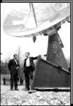
![[Doc Ewen looks into the horn antenna, 1950]](ewen_horn1s.jpg)
|
|
Image courtesy of Doc Ewen
|
Introduction
Harvard Cyclotron: 1948-1951
Detection of HI Line: 1951
Harvard 24ft and 60ft and NRAO founding: 1952-1956
1950s and 1960s: Two Roads that Crossed
Microwave & Millimeter Wave Applications in the 1970s and 1980s
Mm Wave Radiometry in the 1990s
May 2001 visit to NRAO Green Bank
Bibliography
Permissions
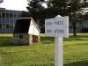
![[Doc Ewen and horn antenna, 2001]](ewen_horn2s.jpg) |
| Image courtesy of Doc Ewen |
|
Doc Ewen: The Horn, HI, and Other Events in US Radio Astronomy
by Doc Ewen, © 2003
Slide Presentation: Detecting the Interstellar Hydrogen Line, 1951
I prepared these slides for the Interstellar Hydrogen Workshop, held at NRAO in Green Bank WV in May 2001. At the Workshop I presented the chronology of events during 1950 and early 1951 that led to the "discovery" of the hydrogen line. Most of my time during that year was spent at the Harvard Nuclear Research Lab, just down the street from the Lyman Lab where I was assembling the hydrogen radio telescope on the weekends.
(Click on the thumbnails for larger photos and fuller explanations.)
|
Slide 1 provides a brief summary of my two projects in 1950 and my approach to completing both of them. The external cyclotron beam was obtained on February 16, 1951 and the Hydrogen Line the following month on March 25th (Easter Sunday).
|
| |
|
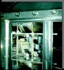
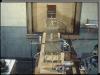
Slide 2 is a photo of the external beam machine installed in the Cyclotron, which consists of a beam scatterer, and the magnetic channel that accepts the scattered particles and directs them out of the cyclotron. The scatterer is shown in greater detail in the next slide. The magnetic channel was made in four sections coupled together to provide a continuous path from the entrance to the exit. Each section was remotely controlled to allow position adjustments without disturbing the internal vacuum. The channel sections could not be moved when the magnetic field was on. Turning the field on or off required a few minutes. Removing the side plates of the cyclotron chamber to make mechanical adjustments, followed by reinstallation of the plates and evacuation of the chamber, required about one week. The design allowed mechanical adjustments while the field was off. Mechanical adjustment of the four section channel was further enhanced by locating a Lucite rod at the end of each channel to intercept the beam. The resulting scintillations were measured by a scintillation counter integrated with a Lucite rod such that the rods could be introduced or removed while the cyclotron was in operation. In this manner, each of the four sections of the magnetic channel could be adjusted separate of the others. The position of the scatterer could also be adjusted while the cyclotron was in operation. The appropriate order in which to make the several adjustments was itself a challenge. The magnetic channel was designed to shunt the field of the cyclotron by guiding it through the walls of the channel to provide a central path with a low magnetic field. The particles escaped and formed an external beam when released from the magnetic field of the cyclotron.
|
| |
|
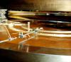
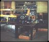
Slide 3: this photo is among my favorites: it shows the scatterer. The heart of the system is a railroad track carrying a very special car. An aluminum rod passes through the car. Each end is equipped with spring fingers. Those in the foreground engage the pole of the magnet. Those in the background engage a curved aluminum plate supported on a curved plastic plate, to electrically isolate the aluminum plate from the pole of the magnet. A battery and potentiometer provided a controlled current to be passed through the rod. With the field on, the direction of current flow in the rod causes the railroad car to move in either direction. The location of the car on the track was measured by introducing a string of resistors in series along the track. The junction between resistors was mechanically sensed by a wiper. The position of the car was determined by an ohmmeter circuit. The actual particle scatterer is the vertical rectangular piece of aluminum mounted on the circular drive mechanism located near the end of aluminum rod in the foreground. The outward radial position of the scatterer is adjustable by rotating its off-center mount about a vertical axis. Rotation of the off-center mount is accomplished with the aid of a solenoid driven pin which engages the ratchet controlled shaft of the off-center mount. This adjustment is made with the cyclotron field off, but with the vacuum intact. This gadget is one of my favorites because a visitor to the Cyclotron Lab asked me one day to describe my approach to the external beam. He was particularly interested in the scatterer. When I described the approach, he was most interested in the track and the railroad car. I mentioned that I had purchased them for a few dollars. He asked for further details. I told him that non magnetic brass cars and tracks are readily available at most hobby shops. He thought that was very innovative. He told me that they used the same railroad car technique, but all the parts were made at considerable expense and time in their own machine shop. He then told me that he was from Chicago and that most people called him Professor Fermi, but he would prefer that I call him Enrico.
There were two other visitors to Lyman Lab, that generated memories. One day a tall fellow dashed into the lab searching for a quick answer to a critical question. I immediately recognized that it was Bob Oppenheimer. He wanted to know how to get to Fenway Park to enjoy an afternoon Red Sox game. Then there was the time that a tall lanky fellow showed up at the front desk of Lyman asking for Doc Ewen. He didn't have to mention his name. Everyone knew it was Ted Williams. He had come by to say hello to his "former Prof from Amherst College." Ted and a few other ball players were students of mine in the Navy V-5 program at Amherst in '42-'43.
|
| |
|
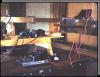
Slide 4: Cyclotron beam exit channel.
|
| |

|
Slide 5: First page of 1944 van de Hulst paper. In the section on "Origins" of a paper titled "Radiogolven uit het wereldruim" [Radio waves from space] given at a colloquium in Leiden in April 1944, published in Nederlands Tidschreift Natuurkunde, December 1945, van de Hulst said, "Discrete lines of hydrogen are proved to escape observation. The 2.12cm line, due to transitions between hyperfinestructure components of the hydrogen ground level, might be observable if the life time of the upper level does not exceed 4.108 years, which however, is improbable."
|
| |
|
Slide 6: First page of 1948 Shklovski paper. In the English translation of a paper titled "A Monochromatic Radio Emission from the Galaxy and the Possibility of Observing It", originally published in Russian in Astronomicheski Zhurnal SSSR 26 (1), 10-14, 1948, Shklovski said, "The experimental possibilities of detecting this emission are discussed. It is shown that with radio apparatus of present day sensitivity, the said emission will be detected if the gain of the antenna is greater than 65, a value easily attainable."
|
| |
|
Slide 7: Later in the same paper, Shklovski says, "To sum up, one may say that with the resources of modern radio techniques it is fully possible to detect and measure the monochromatic radio emission of the galaxy."
|
| |
|
Slide 8: Shklovski's final sentence in the 1948 paper is, "Soviet radio physicists and astronomers should closely concern themselves with the solution of this intriguing and important problem."
My conclusions were: the Dutch will not try detection, the Russians may try detection; I should proceed on the assumption of a negative thesis.
|
| |
|
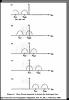
Slide 9: The "switch frequency" technique is a method for detecting weak lines like the hydrogen line. A switch is introduced in the receiver to cause the receiver to tune rapidly (30 Hz) back and forth between two frequencies displaced by 75 KHz (in the case of hydrogen). The two frequencies are then tuned together to move slowly from lower to higher frequencies, beginning at a frequency well below the rest frequency of hydrogen. A synchronous detector in the video circuit assigns a positive output to one frequency and negative to the other. As the two displaced frequencies pass over a line, the output will be positive when the line is at the first receiving frequency and negative when it passes through the second. This (+) followed by (-) feature is referred to as the "S-Curve".
Normally, the switch frequency is applied to the first local oscillator in a superheterodyne mode. For several technical reasons, I elected to switch the second local oscillator in a double conversion superheterodyne. That had its own set of problems, but they were manageable.
|
| |
|
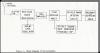
Slide 10: Hydrogen line receiver schematic from doctoral thesis.
|
| |
|
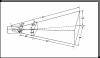
Slide 11: The design of the horn antenna was based on descriptive information presented in the Rad Lab book on Antennas by Sam Silver [Microwave Antenna Theory and Design, edited by Samuel Silver. MIT Radiation Laboratory Series 12, published by McGraw-Hill, 1949; reprinted by P. Peregrinus on behalf of the Institution of Electrical Engineers, 1984]. The maximum size was determined by the geometric constraints of the fourth floor parapet at Lyman Lab. I sent my calculations and sketches to Sam for a sanity check, before sending the build order to the Physics Dept. Model Shop. It was up on the parapet in about three weeks.
|
| |
|
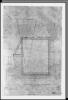
Slide 12: My November 1949 sketch of the horn antenna on the fourth floor parapet of Harvard's Lyman Laboratory.
|
| |
|
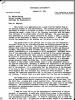
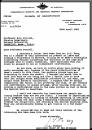
Slide 13: Ed Purcell's January 1950 letter to Harlow Shapley requesting funds from the Rumford Fund of the American Academy of Arts and Sciences.
|
| |
|
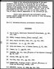
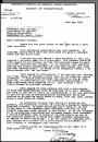
Slide 14: Page 2 of Purcell's funding request letter, with itemized list including antenna ($150), APT-5 xmtr ($100), power supply ($75), mixer parts ($100), and waveguide ($75), for a grand total of $500.
|
| |

|
Slide 15: Grant award letter, February 28, 1950: the check is in the mail! Program kickoff, March 1950. Program completion, March 1951.
|
| |
|
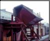
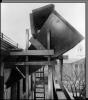
Slide 16: The horn antenna on the fourth floor parapet of Lyman Lab.
|
| |
|
Slide 17: Looking east along the parapet of Lyman Lab.
|
| |
|
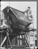
Slide 18: Inspecting the patch work. After one year, parts of the copper skin had cracked and peeled away from the plywood. I purchased fifty feet of rope from a local hardware store, tied one end around my waist and the other to the lower section of the antenna mount. With a large soldering iron, solder, and a bristle brush I went over the side, four floors up, and slid into the horn. About an hour later, I managed to climb out of the horn back on to the parapet. This picture of me inspecting the patchwork was taken about two days later. The line was detected within the next few weeks.
|
| |

|
Slide 19: The mixer. The mixer design was taken from the Rad Lab book on Mixers by Bob Pound [Microwave Mixers, by Robert V. Pound. MIT Radiation Laboratory Series 16, published by McGraw-Hill, 1948]. The mixer shown in the book operates at S-Band, hence, the scale factor was approximately 2 X. Bob was very helpful on this matter, as well as on many others. He is the type of fellow you like to have around when youre building a hydrogen line receiver. On a visit to the Bell Telephone Research Lab at Homdel, NJ, suggested by Purcell, Harold Friis gave me (in his words) "two of the best 1N21 crystals ever tested". They were measurably better than any in the batch I had scrounged from my friends on Vassar St. at MIT. One was in the receiver on the night of March 25, 1951.
|
| |
|
Slide 20: The mixer, in the foreground, is connected to the throat of the horn via a slotted line.
|
| |
|
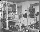
Slide 21: A general view of the receiver, taken from the door into the room. The throat of the horn (not shown) enters from the left through the window.
|
| |
|
Slide 22: The throat of the horn antenna enters at the right. The gas discharge noise source in the foreground is hung by a rope from the ceiling.
|
| |

|
Slide 23: A fortuitous event: Report cover of Bill Mumford's gas discharge noise source for noise temperature calibration of the hydrogen line receiver, June 1949. [A Broad-Band Microwave Noise Source, by W.W. Mumford. Bell Telephone System Monograph 1721, also published in Bell System Technical Journal vol. 28, p. 601-618, 1949.]
|
| |
|
Slide 24: Noise source for calibration of the 21cm receiver.
|
| |
|
Slide 25: The final configuration of the receiver, 1951.
|
| |

|
Slide 26: Doc Ewen and the receiver at the time of detection.
|
| |

|
Slide 27: The classic "S-curve" of the switch frequency receiver. Copy of data record obtained on April 9, 1951, about two weeks after first detection.
|
| |
|
Slide 28: Letter from Joseph Pawsey to Ed Purcell, April 20, 1951. Frank Kerr, teaching at Harvard while on leave from CSIRO Division of Radiophysics, had written to Pawsey of the detection. At Purcell's suggestion, I went to the Harvard Observatory, in mid April, to meet and talk to Van de Hulst for the first time, and to tell him about the discovery. Ed told me that Van de Hulst was teaching a course at Harvard during the spring term. It was the same course that he taught at Leiden, during the prior fall term. When I met with Van de Hulst at the Observatory he called Oort, and I talked with Oort for nearly an hour describing the switch frequency technique. This was the first time that we learned the Dutch had been searching for the line for several years. Had we known, we would not have tried.
|
| |
|
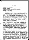
Slides 29-30: Letter from Purcell to Pawsey, May 9, 1951, describing the equipment, the results, and future equipment needs. On page 2 of the letter, Purcell says, "I think we ought to send a letter to the Physical Review or Nature (probably the latter) fairly soon.... We will allow time for a reply to this letter before sending anything off."
|
| |
|
Slide 31: Letter from Pawsey to Purcell, May 18, 1951. Pawsey appreciates the description of technique, and notes that their first observations will be "tonight". He agrees with Purcell about sending a short note to Nature, and appreciates the confirmation opportunity. He mentions the large number of radio astronomy papers that have appeared in the Australian Journal of Scientific Research, Series A (Physical Sciences) and suggests that journal as a possible place for a longer paper on the detection. He sends congratulations to Ewen.
|
| |

|
Slide 32: Ed Purcell, Taffy Bowen, and Doc Ewen.
|
| |
|
Slide 33: Doc Ewen and Ed Purcell with the horn, at the dedication of the Harvard 60ft antenna in 1956.
|
| |
|
Slide 34: The horn antenna today, outside NRAO's Jansky Laboratory in Green Bank, WV.
|
| |
Editor's note: In these slides and on the related text page Ewen describes the equipment, the detection of the HI line, and events surrounding that detection. For a more detailed account of the methodology and results, see the initial detection papers as well as the 1999 description of the detection:
- "Observation of a Line in the Galactic Radio Spectrum." H.I. Ewen and E.M. Purcell, Nature 168: 356, 1951.
- "The Interstellar Hydrogen Line at 1420 Mc./sec, and an Estimate of Galactic Rotation." C.A. Muller and J.H. Oort, Nature 168: 357, 1951.
- See also the note by J.L. Pawsey at the end of the paper by Muller and Oort. The Australian results were published more fully later: Australian Journal of Scientific Research A5: 437, 1952.
- "How Ewen and Purcell Discovered the 21 cm Interstellar Hydrogen Line." K.D. Stephan, IEEE Antennas and Propagation Magazine 41 (1): 7-17, 1999.
Modified on Tuesday, 23-Aug-2005 08:56:44 EDT by Ellen Bouton
|
